
Contents
Same energy, different supply requirementsWhy electricity bills also account for capacityHow time changes a peakHow to lower the peakFrom a lower curve to a lower bill
Same energy, different supply requirements
The familiar starting point on an electricity bill is energy consumption in kilowatt-hours, or kWh. Yet a total of 20 kWh leaves an important question open: was that energy used within one hour, or spread over several? The power needed at the same time can differ even when total consumption is equal.[3]
Consider two devices, each drawing 10 kW and needing to run for one hour. Starting both together uses 20 kWh in one hour and requires 20 kW of combined power. Running them in sequence still uses 20 kWh, now over two hours, while the combined peak is only 10 kW. The second arrangement takes longer to finish all tasks and halves the highest simultaneous power requirement.
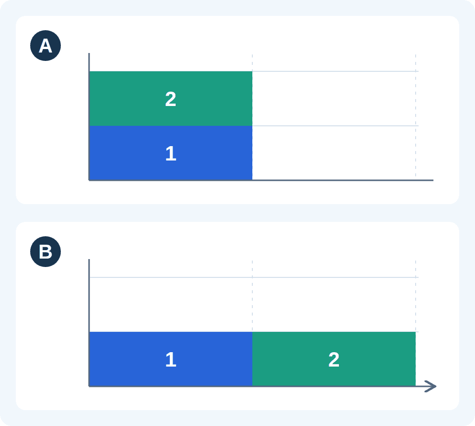
A · Run together: 20 kW for one hour
The devices overlap, drawing a combined 20 kW and consuming 20 kWh in the first hour. Both are off during the second hour.
B · Run in sequence: 10 kW for two hours
Each device runs for one hour in turn. Combined power stays at 10 kW, and total energy is still 20 kWh. Equal areas correspond to different peaks and durations.
Author-created illustration calculated from the relationship between power and energy [3], rather than measurements. Each device runs at constant power and can start at a different time. There are no other loads or local sources; startup effects and efficiency changes are ignored. Both arrangements use the same two-hour comparison period. If both tasks must finish within one hour, B is infeasible.
Time makes the difference visible. Energy accumulates as power is used over time. In Figure 1, energy is the colored area, simultaneous power is its height and duration is its width. Peak shaving addresses the high points of this curve. It can do so while leaving the total task and total energy unchanged.
Why electricity bills also account for capacity
The supply system must deliver power when it is needed. Both arrangements consume 20 kWh, but supporting 20 kW at once calls for a different level of supply capability from supporting 10 kW. US DOE billing guidance explains that higher demand requires utilities to build and maintain more infrastructure to deliver power. This helps explain why a bill can include both energy-based charges and charges linked to power or capacity.[1]
An energy charge accounts for cumulative consumption. Contracted or subscribed capacity specifies an agreed level of power and may determine a basic or fixed charge. A February 2026 residential tariff example published by the French regulator CRE lists an annual fixed component by subscribed kVA band alongside a separate price per kWh. This is one specific way of charging for capacity and energy separately.[4]
The agreed capacity, measured maximum demand and billed demand are distinct quantities. The first is set in advance by the contract. The second is measured over the relevant period. Tariff rules determine the demand used for billing. Some bills charge by contracted capacity band; others also charge for measured maximum demand or apply further conditions. Understanding which quantity a charge uses is essential to assessing the effect of a lower peak.[1][5]
Units also follow the contract. kVA measures apparent power and kW measures real power; power factor relates the two. The French example uses kVA subscription bands. Taipower’s published definitions distinguish installed-capacity contracts expressed in kVA from demand contracts based on fifteen-minute average kW. The examples here use kW for simultaneous real power; an actual contract determines the applicable capacity unit.[1][4][5]
How time changes a peak
Time has two connected roles. Overlap and duration determine the shape of demand: which tasks coincide, and how long high power lasts. The time of day also matters, because prices and grid conditions vary. Moving a task to a cheaper period can change its energy cost; separating overlapping tasks can lower simultaneous demand. These effects may occur together or independently.[1][6]
Demand used for billing is also measured over a defined interval. A US demand-charge survey describes a common method: taking the highest average power over a specified interval within the billing period, often fifteen minutes. The applicable tariff sets the actual interval and charge.[2]
For an explicitly defined fifteen-minute interval, importing 5 kWh gives an average of 20 kW; importing 2.5 kWh gives 10 kW. These values follow from dividing energy by time. A brief spike affects the average differently from power sustained for the full interval. Electrical operation must also remain within actual phase-current, wiring and equipment limits.[1][3]
How to lower the peak
Three methods can be compared using the same starting load: change task timing, reduce equipment power, or supply part of the demand locally. Each can lower the peak at the grid connection, with different operating changes and tradeoffs.
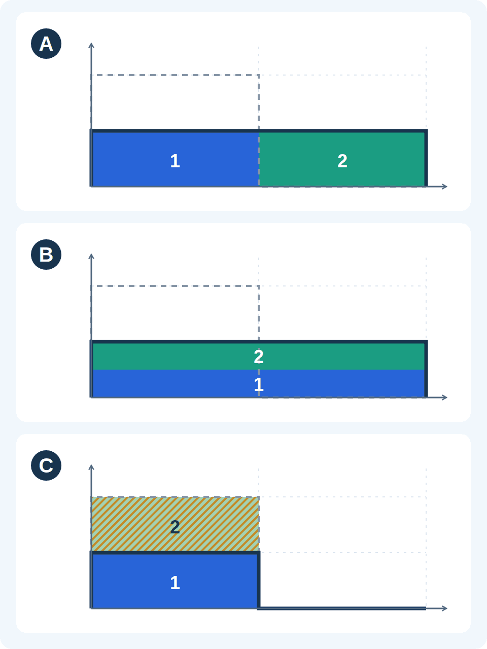
A · Reschedule tasks: reduce overlap
Device 1 runs during the first hour and device 2 during the second. Each still draws 10 kW, but their combined peak falls to 10 kW. Total energy remains 20 kWh, with all tasks completed after two hours.
B · Reduce power: spread the task over more time
Both devices run at 5 kW for two hours, drawing 10 kW together. This example assumes that the devices support power adjustment and can still complete the original tasks. Real processes may experience changes in output, temperature or efficiency.
C · Use local supply: share the power requirement
The devices still draw a combined 20 kW during the first hour. The battery supplies 10 kW and the grid supplies the other 10 kW. Gold hatching represents the battery’s 10 kWh contribution to the shared supply, rather than a dedicated supply to device 2.
Author-created examples based on the control mechanisms and power balance in [6][7][8]; these are not measurements. Other loads, startup effects and efficiency changes are ignored. A and B require tasks that can be delayed or run at reduced power. C requires sufficient available battery energy and discharge power. Recharging is outside the chart; storage losses affect imports over the full charge–discharge cycle.
Where tasks can wait, Figure 2 A reduces overlap by changing their operating times. EV charging may use spare time during a parking session: charge some energy first, then continue after other equipment switches off. That flexibility comes from the actual time available. A vehicle close to departure may miss its energy target if charging power is reduced. US DOE managed-charging guidance considers facility demand, power limits and vehicle requirements together.[7]
Another approach lowers the power of adjustable equipment or temporarily curtails tasks that can be interrupted. The curve drops, while tasks may take longer or affect production and temperature. If all deferred tasks resume together, their demand can overlap again, so recovery needs to be part of the schedule.[6][7]
When both devices must operate together, local resources can share the supply requirement. In Figure 2 C, the devices need 20 kW in total. A battery delivering 10 kW for that hour leaves the grid to supply the other 10 kW. Device demand remains unchanged while net grid imports fall. The battery must deliver 10 kWh and have sufficient discharge power and available energy at that time.[8]
The battery then needs recharging, with losses during charging and discharging. A lower import peak can therefore accompany higher total grid energy use. Recharging alongside other loads can also raise a later peak. Peak-shaving capability depends on preparation before the event and recovery afterwards, as well as what can be delivered during the peak.[8][9]
From a lower curve to a lower bill
A charge based on the highest demand in a billing period must be assessed across all relevant intervals. Reducing one 20 kW event may leave the maximum unchanged if another interval still reaches 20 kW. The billing result follows the highest applicable interval, rather than a single improved reading.[1][2]
Where the fixed component follows a contracted or subscribed capacity band, peak shaving may make a lower band feasible. The contract still needs to be changed, and normal tasks, recovering loads and the required margin must fit within the new limit. In the French subscription example, the fixed charge follows the selected contractual band.[4]
Energy charges continue to follow actual kWh and the applicable time-of-use prices. With equal total consumption and an unchanged price per kWh, spreading demand over time leaves the energy charge unchanged. Capacity and demand charges follow their own rules. The central task of peak shaving is to arrange the same work over time so that less power is required from the grid at the high point, while still meeting completion requirements.
References
- [1] Understanding Your Utility Bills: Electricity — US DOE / Better Plants; Official training material; no overall publication date shown; file path dated 2021-11; printed pages 14–21; checked 21 October 2026
- [2] Identifying Potential Markets for Behind-the-Meter Battery Energy Storage: A Survey of U.S. Demand Charges — NREL; NREL/BR-6A20-68963, August 2017; average demand and capacity-cost mechanisms
- [3] Glossary / Electric — US Energy Information Administration (EIA); Online glossary; kW and kWh entries; checked 21 October 2026
- [4] Comprendre les tarifs réglementés de vente d'électricité (TRVE) — Commission de régulation de l’énergie (CRE), France; Page updated 20 January 2026; tariff structure illustrated for residential subscriptions up to 15 kVA from 1 February 2026; no current price quotation
- [5] About Us: definitions reproduced from Article 3 of the business rules — Taiwan Power Company (Taipower), electronic billing service; Page dated 16 October 2019; definitions reproduced from Article 3 of the business rules; installed-capacity contracts, demand contracts and maximum demand; checked 21 October 2026
- [6] Demand Response and Time-Variable Pricing Programs — US DOE / FEMP; Load curtailment, shifting and time-variable prices; no overall update date shown; checked 21 October 2026
- [7] Managed EV Charging for Federal Fleets — US DOE / FEMP; Control objectives and vehicle requirements; no overall update date shown; checked 21 October 2026
- [8] An Overview of the Automated Dispatch Controller Algorithms in the System Advisor Model (SAM) — Nicholas DiOrio / NREL; NREL/TP-6A20-68614, 2017; SAM 2017.1.17; power balance, energy and recharging constraints
- [9] Solar Integration: Solar Energy and Storage Basics — US DOE / Solar Energy Technologies Office; Storage losses, power and energy; no overall update date shown; checked 21 October 2026